By Ben Edelman, Ezra Edelman, Surbhi Goel, Eran Malach, and Nikos Tsilivis
This post is based on “The Evolution of Statistical Induction Heads: In-Context Learning Markov Chains” by Ben Edelman, Ezra Edelman, Surbhi Goel, Eran Malach, and Nikos Tsilivis.
Machine learning works based on the inductive principle that patterns in the training data are likely to continue to hold. Large language models are induction machines—during training, they gobble up billions of words of text, extracting myriad patterns that can be used to predict the next token. But part of what makes LLMs so powerful is that they don’t only exploit patterns from their training data—they also make use of patterns in the prompt itself. This in-context learning (ICL) ability is what enables LLMs to perform a task based on a few demonstrations, to mimic the style of a piece of writing, or to repeat key phrases from a prompt, all based on the principle that patterns in the context are likely to continue to hold. While the assumption that patterns encountered during training will generalize at inference time is essentially baked into the training procedure, the corresponding in-context claim is something the LLM needs to learn (by induction) during training.
We will focus in particular on a sub-circuit motif called an induction head which researchers have found is responsible for performing some ICL computations in transformer LLMs. Induction heads define a circuit that looks for recent occurrences of the current token, and boosts the probabilities of tokens which followed the token in the input context. They have been shown to emerge when training on a large corpus of language, and contribute to in-context learning abilities. In this work, we aim to study the formation of induction heads in isolation, by introducing a synthetic task, ICL of Markov chains (ICL-MC), for which an optimal solution can rely solely on induction heads.
The task
Markov chains are stochastic processes whose evolution depends only on the present and not on the history of the process. They naturally model many stochastic systems that exhibit the aforementioned property of memorylessness and their applications can be found in many disciplines, from economics to biology. In the beginning of the 20th century, Andrey Markov, the Russian mathematician who introduced them, used them for studying grammatical patterns in Russian literary texts. In 2024, it is our turn to use them for studying LLMs.
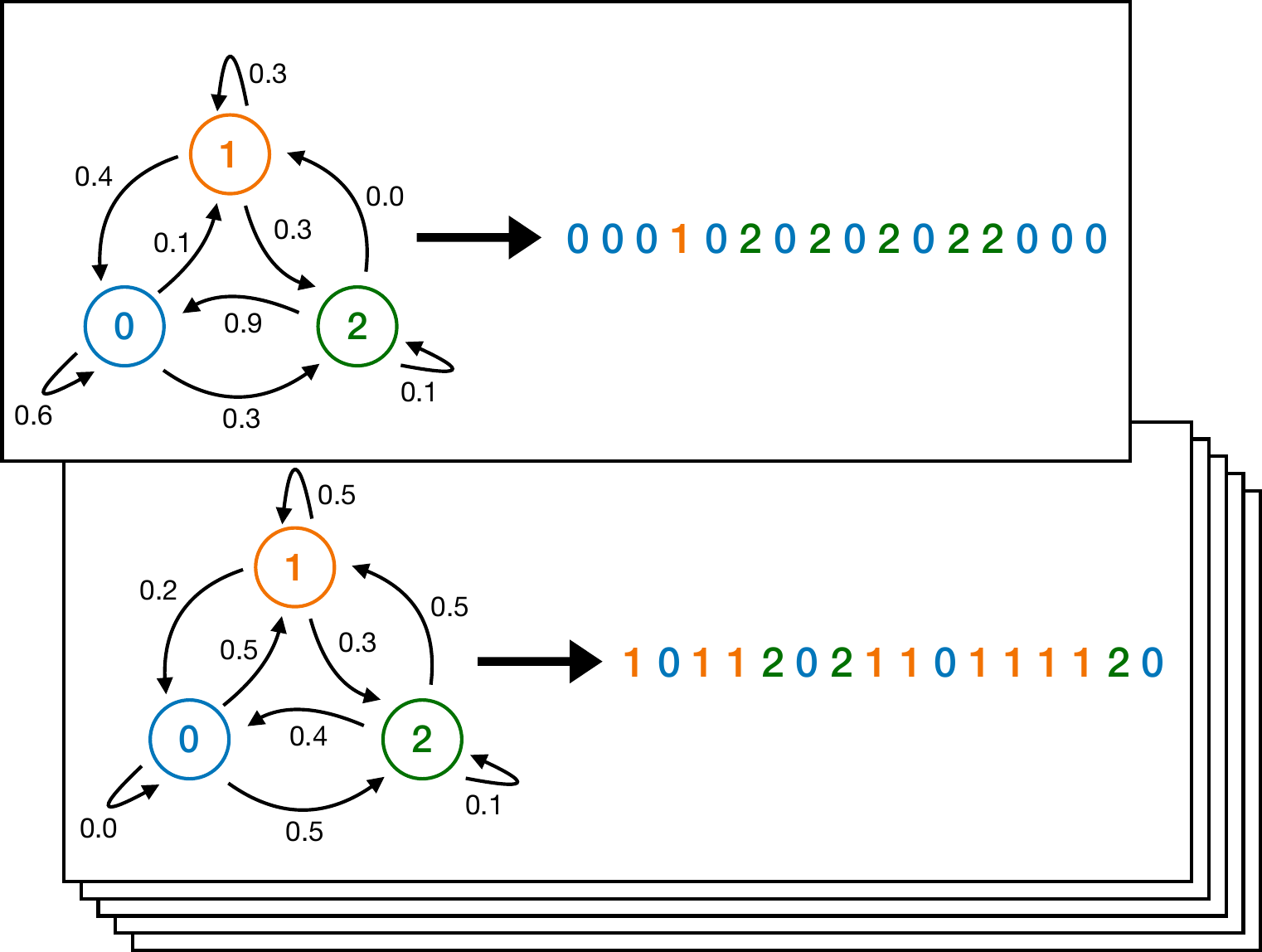
To generate each training (or test) sequence in our ICL-MC task, we first sample a Markov chain from a prior distribution. A Markov chain with k states is described by a transition matrix that gives the probability of transitioning from state i to state j for all states i and j. Then we sample a sequence of tokens (states) from this Markov chain. Here are a few examples of Markov chains, and sequences drawn from them:
Potential strategies
The plan is to train simple two-layer attention-only transformers (with one head per layer) to perform next-token prediction on these sequences, and observe how they leverage the information in their context. For instance, assume we have the following sequence generated by a Markov chain with three states:
What would be your guess for the next state? Alice’s strategy is to choose at “random” and assign equal probability to all 3 symbols. Bob’s strategy is to count the frequency of the states in the sequence so far and simply estimate the probability of each state to be proportional to this frequency count. State 1 has appeared more times in this sequence, and is therefore assigned a higher probability according to this strategy. Carol, on the other hand, finds previous occurrences of the current state (2), counts the number of times this was followed by a state j and assigns this as the probability of the next token being j. In this case, 0 and 1 would have equal probabilities (equal counts). As can be seen in the above Figure (in which this is the second example), the real generated state was 0, so Carol was closer to being right. In general, Carol’s strategy feels more natural for sequences that are generated by Markov Chains and, indeed, when transition matrices are drawn uniformly at random, a version of Carol’s strategy that suitably accounts for the prior distribution is the optimal solution—see Section 2 in the paper for more details.
What does the transformer do?
However, we are not interested in how humans predict tokens, but how transformers do so. Let’s begin our exploration by observing the loss curve of a transformer trained online on ICL-MC:
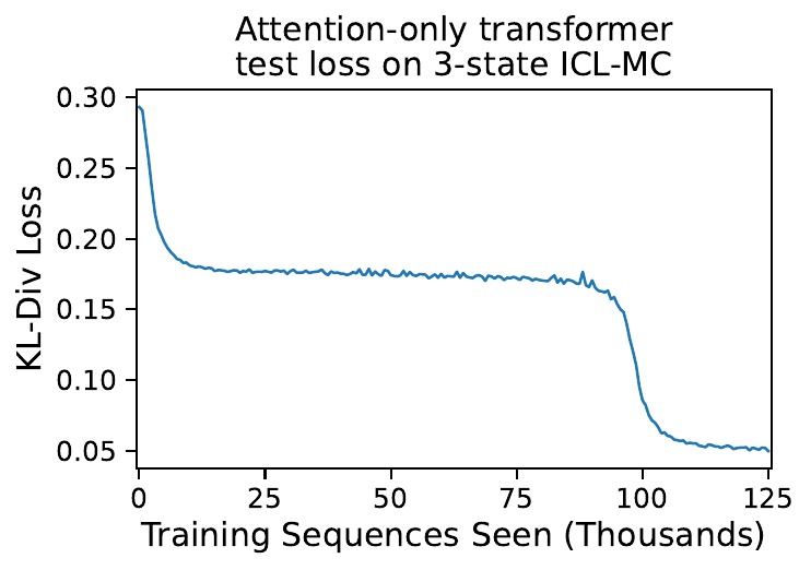 Intriguingly, we see what looks like multiple phase transitions! After an initial period of rapidly falling loss, there is a long plateau period where the model barely improves, followed by a second rapid drop to very low loss.
Our hypothesis was that the network might be starting out with Alice’s “uniform” strategy; then adopting Bob’s “unigram” strategy for a long time, before it finally converges to Carol’s optimal “bigram” strategy. We can test this hypothesis by measuring the KL divergence between the predictions of each strategy and the predictions of the model over the course of training:
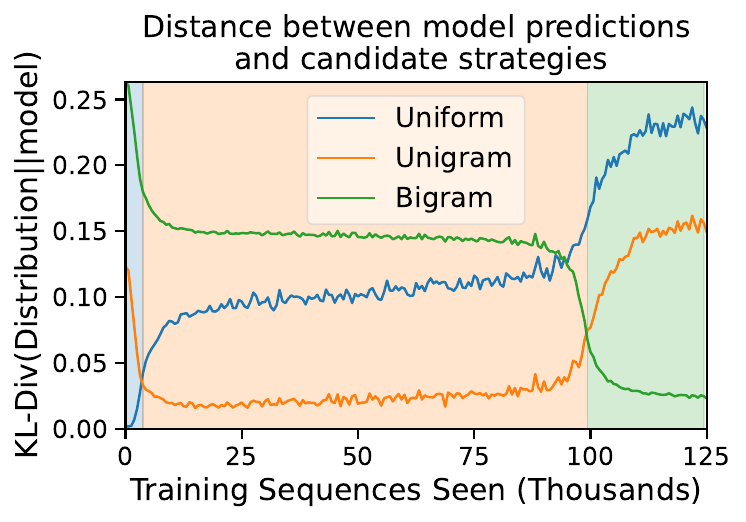
In this plot, the blue curve, corresponding to the distance between the model’s solution and the uniform strategy, starts off at zero—indicating that this is the solution at initialization. Then, the orange “unigram” curve drops near zero and stays low throughout the long plateau, indicating that the model’s predictions are explained by the unigram solution. Finally, at the same time as we saw the final phase transition in the loss curve, the orange curve rises and the green “bigram” curve drops, which tells us that the model has landed near the bigram solution. The background is shaded according to which solution the model is closest to at any particular time. In short, we have validated the hypothesis!
How does the transformer do it?
The KL divergence plot told us about the functional behavior of the network, but it didn’t tell us how the network implements its solutions. To gain some mechanistic insight, let’s peer into the network’s internal attention weights for a single example input:
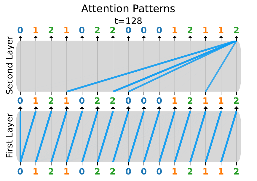
In this video, the blue lines indicate the amount that the token positions on top attend to the positions below, in each layer. For clarity, in the second layer we only show the attention weights from the final token in the sequence.
The attention patterns appear to have sudden changes concurrent with the phase changes we’ve already observed. Most notably, during the second (and final) drop in loss, we see some very structured patterns:
- In the first layer, each token attends to the one preceding it.
- In the second layer, the 2 attends to all tokens that immediately follow a 2.
These patterns are exactly what we would expect of an induction head! It appears that the network learns to implement an induction head in order to perform the bigram strategy. We refer to this as a statistical induction head because it is not just copying tokens—it is predicting the next token according to the correct conditional (posterior) probabilities, based on bigram statistics. For more details, see the paper.
Stepping stone or stumbling block?
We have observed an example of simplicity bias–the network tends to favor the simpler but less accurate unigram solution earlier in training before arriving at the more sophisticated and accurate bigram solution. We can ask: does the existence of the somewhat-predictive unigram solution facilitate faster learning of the bigram solution, or does it distract from the bigram solution, delaying its onset? In other words, is the unigram solution a stepping stone or a stumbling block?
In order to approach this question, we consider two extreme types of Markov chains:
- Doubly stochastic: Markov chains with a uniform stationary distribution—i.e., the transition matrix is doubly stochastic.
- Unigram-optimal: Markov chains where the next state is independent of the current state—i.e., all the rows of the transition matrix are the same.
For doubly stochastic Markov chains, the unigram solution is no better than the trivial uniform solution, because the expected frequencies of the different states are always the same (note that in all our experiments, we sample the initial state from the Markov chain’s stationary distribution). For unigram-optimal Markov chains, as the name suggests, the unigram solution is optimal, because the bigram statistics are entirely determined by the unigram statistics.
First, let’s see what happens when we train our transformer on only doubly stochastic Markov chains, and evaluate on our original full distribution over Markov chains:
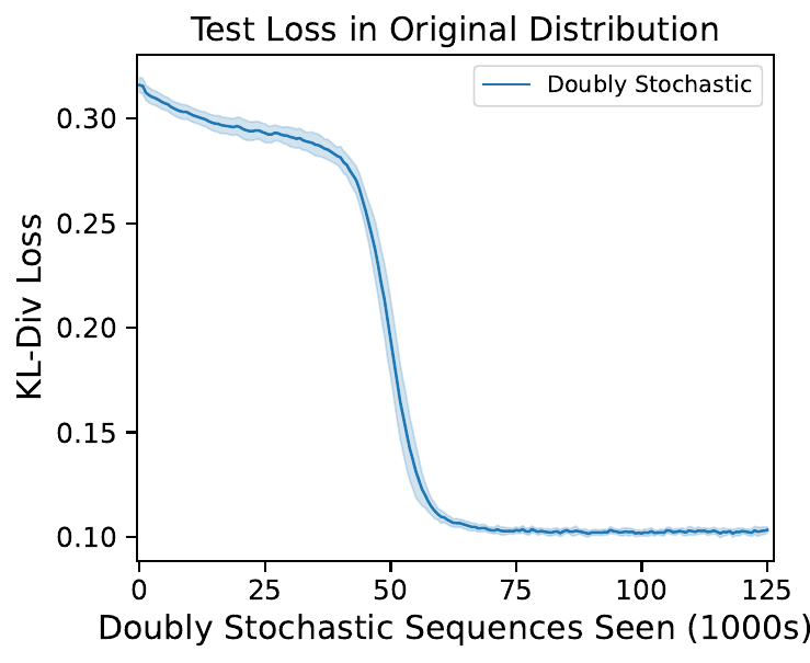
The model still generalizes quite well on the full data distribution even though it has been trained only on a small slice of it. Unsurprisingly, there is no intermediate unigram plateau (there is only one phase transition instead of two). By inspecting the final attention weights, we can see that the network has indeed learned an induction head:
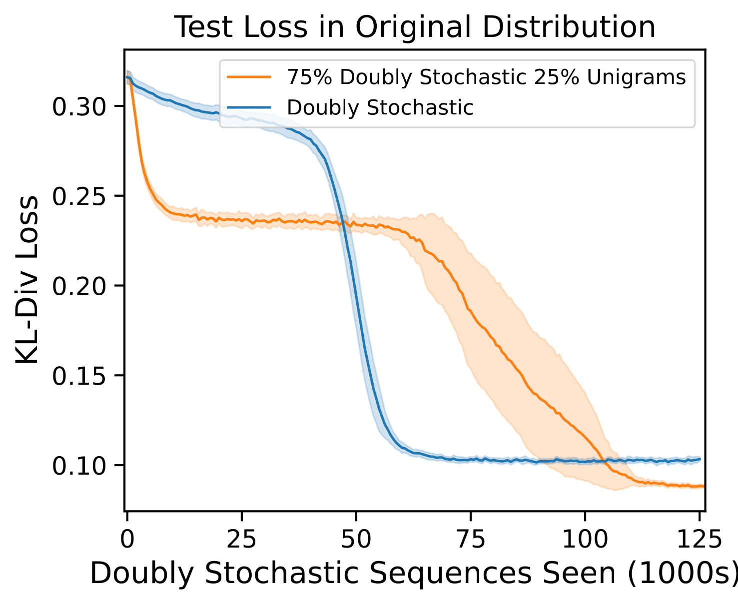
Now, let’s try mixing in some unigram-optimal Markov chains into the training distribution:
 |
|---|
| Comparison between transformers trained on the two distributions. In the doubly stochastic distribution, transition matrices are uniformly random 4x4 doubly stochastic matrices. In the unigram distribution, every row in the transition matrix is the same, and is uniformly random over probability vectors of length 4. The error bars are 95% confidence intervals calculated over 10 distinct random seeds (which randomize initialization and data sampling), and the lines denote the mean loss over the seeds. For each seed, the same doubly stochastic sequences are used in both the pure doubly stochastic distribution, and the mixture distribution. |
The X-axis scale only counts training sequences that came from doubly stochastic Markov chains, so the unigram-optimal sequences we’ve mixed in are “free” additional training data. It appears that adding in these bonus unigram-optimal sequences delays the formation of the induction head. This is evidence that the intermediate solution is a stumbling block, not a stepping stone to the correct solution. (At the same time, these bonus sequences do seem to lead the network to converge to a somewhat lower final loss.)
Mathematical analysis
Due to its simplicity, our learning setup is amenable to mathematical analysis of the optimization process. This provides numerous insights into how the model passes through the different strategies and what happens to the different components of the transformer during training. In particular, in a simplified linear transformer architecture, we find that, starting from an “uninformed” initialization, there is signal for the formation of the second layer, but not for the first. However, once the second layer starts implementing its part, the first layer also starts to click. We suspect that this coupling is responsible (at least partially) for the plateaus and the sudden transitions between stages. Our analysis further elucidates the role of learning rate and the effect of the data distribution. For both our theory and our experiments, we used relative positional encodings. The analysis suggests that there should be a curious emergent even-odd asymmetry in the first-layer positional encodings during training, and we confirmed this empirically in the full transformer as well! See the paper for more details.
A Markov ICL renaissance
Reflecting how natural our setting is, in parallel with our work several independent groups have released exciting papers studying similar problems in language modeling. Akyürek et al. study how different architectures (not only transformers) learn to in-context learn formal languages, which in some cases correspond to n-Markovian Models (n-grams). Their experiments with synthetic languages motivate architectural changes which improve natural language modeling in large scale datasets. Hoogland et al. document how transformers trained on natural language and synthetic linear regression tasks learn to in-context learn in stages, implementing different strategies at each stage. Makkuva et al. also argue for the adoption of Markov Chains to understand transformers and in their paper they study the loss landscape of transformers trained on sequences sampled from a single Markov Chain.
Perhaps closest to our work, Nichani et al. introduces a general family of in-context learning tasks with causal structure, a special case of which is in-context Markov chains. The authors prove that a simplified transformer architecture can learn to identify the causal relationships by training via gradient descent. They draw connections to well known algorithms for this problem, and also characterize the ability of the trained models to adapt to out-of-distribution data. There are many cool similarities (and differences) between their and our work—we hope to discuss these in more detail in the next version of our paper. In-context learning Markov Chains (or more general Markovian models) with language models seems to us to be a fruitful task for understanding these models better, and we are excited by the recent burst of activity in this direction! (apologies if we missed your recent work!)
Bonus: trigrams and more
A natural follow up is to study processes where the state can depend on multiple preceding tokens, not just one—n-grams, not just bigrams. It is straightforward to extend our training distribution in this way, by sampling transition matrices with rows corresponding to tuples of states.
When we train our two-layer transformer on n-gram distribution, it bottoms out at the performance of the bigram strategy, which is suboptimal for n>2. But if we increase the number of attention heads in the first layer from 1 to n-1, then the model achieves dramatically lower loss! Under the hood, the different first-layer heads are specializing: one head looks back by 1, another head looks back by 2, and so on, so that together they look at the previous n-1 tokens. Experimentally, the models still learn in phases, working up from unigrams, to bigrams, to trigrams, all the way to n-grams!
In the following videos, the different colors in the first layer attention visualization correspond to different heads.
Check out our paper!